Introduction
Explainability of machine learning models is a hot topic right now - particularly in deep learning where models are that bit harder to reason about and understand. These models are often called ‘black boxes’ because you put something in, you get something out and you don’t really know how that outcome was achieved. The ability to explain machine learning model’s decisions in terms of the features passed in is both useful from a debugging standpoint (identifying features with weird weights) and with legislation like GDPR’s Right to an Explanation it is becoming important in a commercial setting to be able to explain why models behave a certain way.
In this post I will give a simplified overview of how LIME works (I may take some small technical liberties and manufacture some contrived examples to demonstrate some of these mechanisms and phenomena - apologies) and then I’ll give a brief explanation of how LIME can be applied to a sci-kit learn SVM-based sentiment model and then a huggingface/torch sentiment model.

understanding individual contributions of words is useful when working with NLP Classification Models
Understanding LIME
Lime stands for Local, Interpretable Model-agnostic Explanations and is a technique proposed by Ribeiro et al. in 2016. The basic premise is that for a given input example (in an image classifier we’re talking 1 image, in a text classifier we’re talking 1 unit of text e.g. a paragraph or a sentence, in a numerical model trained on tabular data we’re talking 1 row from that table), LIME can approximate how much of an effect each of the features extracted from the input have on the final output (i.e. How important are a cluster of pixels in an image?, How important are specific words/phrases in a sentence?, How important is each column in that row of numbers?).
For a given example both contributing and negating features are highlighted (reasons for and against that decision).

Figure 1 from the Ribeiro et al paper giving an overview of how LIME works
Local
The local aspect of LIME is described in the paper:
…Although it is often impossible for an explanation to be completely faithful unless it is the complete description of the model itself, for an explanation to be meaningful it must at least be locally faithful, i.e. it must correspond to how the model behaves in the vicinity of the instance being predicted…
This is a really important constraint of LIME: it offers excellent example-specific explanations that work well for pockets of similar data points but these explanations can’t necessarily be generalised for the whole of the model under examination. The authors of the paper also attempt to illustrate this limitation in a diagram:

Figure 3 from the Ribeiro et al attempts to illustrate how LIME can offer explanations within a local neighbourhood of data samples
To Spam or not to spam: that is the question
This is especially important in tasks that are highly context dependent (like text classification). Here’s a contrived example of a spam detection use case. Take the words “7 million usd” as in:
Sir,
I am a wealthy widow and if you help me I will pay you 7 million usd
Best Regards
and also
Kevin,
the new term sheet from the investors is in, they’re offering 7 million usd for 5% equity,
Brian Smith
Head of Mergers & Acquisitions
In the first example, the words “7 million usd” contribute to the suspicion that this is a scam in the presence of “wealthy widow” and “help me”. In the second example the words “7 million usd” aren’t as important, they’re words that you’d probably expect in a legitimate email about an investment opportunity from your colleague in Mergers.
The point I’m trying to make is that it’s very difficult to come up with good general rules about which words are important without any context (and indeed if you can do that then you probably don’t need machine learning, you can just build a rule-based system that checks for the presence or absense of words on a list). The overall decision function of “spam or not spam” is much more complicated than “these words are good and these words are bad” but for a certain set of “spammy” examples we can certainly say which words are more spammy and which words are less spammy. This is analogous to the concepts at play in LIME too.
Therefore when we’re using LIME, we should avoid saying things like “The model seems to consider the words ‘million’ and ‘usd’ spammy” and we should say things like “in cases similar to the widow email, it looks like the words ‘million’ and ‘usd’ contributed to the decision that this email was spam in the absense of any other redeeming words”.
Interpretable
Some machine learning models like linear models and Decision Trees are inherently interpretable through being able to measure parameter coefficients (how big the weight of the feature is when calculating the decision boundary line) in the case of the former and how early on a feature appears in a decision tree (since decision trees use information gain to put features that tell us most about the final classification/decision near the top of the tree so that they impact more data points) in the case of the latter.
LIME exploits these explainable models in order to explain the local context around a given input example. We perturb (slightly change) the input example and use the black-box model under analysis to make predictions. As words are added or removed from the input, the output from the black box model changes slightly (in the [contrived again] example below, removing the word ’love’ from the movie review reduces the probability that the review is positive.)
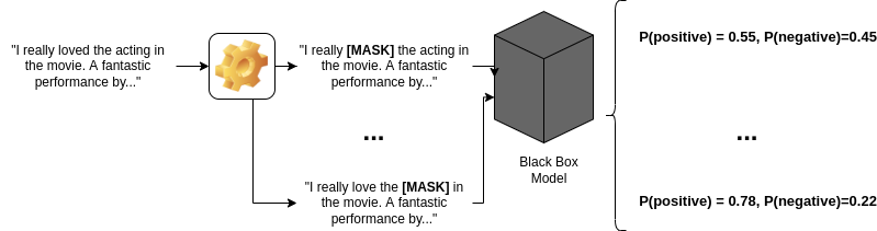
LIME perturbs input examples by changing words around in order to understand the individual contributions of words to an outcome
These perturbed inputs and the outputs from the ‘black box’ model that we’re analysing outputs are then used as a training set to train the local, interpretable model.
For text models, LIME uses Bag-of-Words (BoW) representations of the perturbed input as the features for the local model.
We can then use the interpretable information (parameter coefficients/feature position in decision tree) for the local model to approximately interpret the effect that the different words have on the bigger model since each word in the local BoW vocabulary will have an associated coefficient.
Model-Agnostic
LIME’s model agnosticism is one of its most useful attributes. As long as you know how to encode the input data and your model has the ability to provide probabality distributions over its outputs, you can provide local explanations for any type of model. This is because the explanation comes from the local model and the BoW features therein rather than the black box model.
In the section below I’ve provided some examples of how to use ELI5 with some different types of models.
Explanation
Explanations that are produced by LIME for NLP models are expressed in terms of which words/phrases were considered as the biggest contributing factors towards a class decision by the model.
If you look at the results in Jupyter you’ll get red and green highlights over the text input showing the degree to which each word contributed (green) or reduced (red) the likelihood that the input example is from the class under the microscope. In the example below you can see that kidney stones and medication are keywords that the model has learned can be used to classify examples in this neighbourhood (remember these explanations don’t apply globally) as medical and that the presence of these words detracts from the likelihood that the email is about religion or graphic design.

An example explanation from LIME
The <BIAS> contribution is the model’s underlying bias towards or against a particular class - again *within this neighbourhood. The most intuitive way to think about this parameter is that it describes the model’s perception that other examples, similar to this one, belong to the given class. It is based on the a priori probability that a randomly perturbed sample in the current neighbourhood belongs to each one of those classes since in a well trained model with good features, different parts of the neighbourhood are more likely to correspond to different classes. The bias is usually a much smaller contributing factor than the actual features as we see in the example above.
We can also inspect the weights/feature importances that the model has generated for the current local neighbourhood and see, for each class, what words or phrases the model thinks are predictive of a particular class.

Feature importances example
This table can also be useful as it can highlight surprising/incorrect results like that “to be” or “do anything” might signal a post about atheism. It’s always worth having a look and if you see anything weird then also check whether the model is trustworthy or whether your black-box model might be doing something strange.
Usage Examples
Requirements and Setup
In order to get any of the examples below running you will need a relatively recent version of Python 3 and the eli5 library installed too. You will probably want to run the example code in a Jupyter Notebook so that you can see the pretty graphical explanations.
If you’re not sure about which version of Python to install, you might want to have a quick look at my opinionated guide to Python environment setup.
All of these examples will work fine on machines without GPUs although the transformer model is a little slow running on CPU (it takes about 60 seconds to run on my 2020 Dell XPS w/ i7, 16GB RAM).
ELI5 and Sci-kit Learn
Scikit-Learn is one of the most widely used machine learning libraries used by data scientists everywhere. In this first example we’re going to train a model in sci-kit learn and then use ELI5 to get an explanation for it. Make sure you have your python environment set up and scikit-learn installed.
If you recognise the following example that’s because it is also the example that ELI5 use in their documentation but I’ve added some commentary to what’s happening in the code snippets.
We are going to train a Support Vector Machine (SVM) model to predict which newsgroup an email came from thanks to the 20 newsgroup dataset. SVMs with a linear kernel do have feature coefficients which could be used to provide global feature importance. However, to make it harder we will be using an RBF kernel and we will use Latent Semantic Analysis because that’s the setup used in the example and it’s a combination that cannot be explained simply without LIME.
Why SVM and LSA?
So why do they used RBF and LIME? Is it a contrived example just to show off LIME?
Well LSA is often used as a way to get more performance from an underlying BoW model by reducing dimensionality and combining commonly co-occuring words into a single feature (rather than having one feature per word). With LSA we might be able to do a better job of capturing some of the general ’topics’ and themes that occur across a whole document rather than just tracking words and key phrases (n-grams). This could help with scenarios like the spammer above where LSA could put co-occurences of ‘widow’, ‘million’ and ‘usd’ in one dimension and ’term sheet’, ‘million’, ‘usd’ in another dimension, giving the SVM a bit of context for the words ‘million’ and ‘usd’.
RBF is a SVM kernel that can separate data that is not linearly seperable and there’s a great explanation of this here. RBF is often cited as a reasonable first choice of kernel for SVMs. However, NLP practitioners will generally recommend a linear kernel for text classification as in practice, and in my experience, text is usually linearly separable. However it will always depend on dataset so do some visualisation during exploratory analysis to see if an RBF kernel is appropriate.
Training the Model
First we are going to use scikit-learn’s built in fetch_20newsgroups helper function to download some example emails from 4 newsgroups. There could reasonably be some serious overlap between the atheism and christian boards so this might be where LSA and our RBF kernel come in handy.
from sklearn.datasets import fetch_20newsgroups

categories = ['alt.atheism', 'soc.religion.christian',
              'comp.graphics', 'sci.med']
twenty_train = fetch_20newsgroups(
    subset='train',
    categories=categories,
    shuffle=True,
    random_state=42,
    remove=('headers', 'footers'),
)
twenty_test = fetch_20newsgroups(
    subset='test',
    categories=categories,
    shuffle=True,
    random_state=42,
    remove=('headers', 'footers'),
)
In the next code snippet we train the code. The TFIDFVectorizer splits the texts into tokens, builds a bag-of-words representation of the text but with the addition of TF-IDF information to help us filter out words that don’t give us any information.
The TruncatedSVD object is applied to the TFIDF vectorizer to give us our latent signals/categories.
Then the SVC is fed the output of the SVD/LSA component.
Each component is linked together into a Pipeline object that basically provides syntactic sugar for us later and avoids us having to manually define an interface for ELI5 to call in order to use our model.
Finally we call pipe.fit() on the training data to actually feed the pipeline and train the model and pipe.score() on the test set to give us a top-line accuracy (if we were doing a thorough job we should probably also look at other appropriate metrics).
random_state is simply a number that is used to seed Python’s pseudo-random number generator which
scikit-learn usesfor pseudo-random operations. Setting random state explicitly is a good habit to get
into in order to preserve the reproducibility of your models.
Another key parameter set here is probability=True on the SVM. This will allow us to get the probability distributions
across the classes that LIME will need later. If you don’t set this then predict_proba() will fail at the next step.
from sklearn.feature_extraction.text import TfidfVectorizer
from sklearn.svm import SVC
from sklearn.decomposition import TruncatedSVD
from sklearn.pipeline import Pipeline, make_pipeline

vec = TfidfVectorizer(min_df=3, stop_words='english',
                      ngram_range=(1, 2))
svd = TruncatedSVD(n_components=100, n_iter=7, random_state=42)
lsa = make_pipeline(vec, svd)

clf = SVC(C=150, gamma=2e-2, probability=True)
pipe = make_pipeline(lsa, clf)
pipe.fit(twenty_train.data, twenty_train.target)
pipe.score(twenty_test.data, twenty_test.target)
Getting Some Predictions
Now that the model is trained it is possible to run it on unseen data and get a prediction. In the tutorial the ELI5 authors provide a pretty printing function that shows the probability distribution of the labels for a given example.
def print_prediction(doc):
    y_pred = pipe.predict_proba([doc])[0]
    for target, prob in zip(twenty_train.target_names, y_pred):
        print("{:.3f} {}".format(prob, target))

doc = twenty_test.data[0]
print_prediction(doc)
This is basically just predicting the classes for the given document, which is the first doc in the test set, and then combining the probabilities in the prediction (y_pred) with the class names (twenty_train.target_names).
Getting an Explanation
Getting an explanation of out this model is relatively simple at this point. We simply import the TextExplainer class from ELI5 and fit() it to the document (the first one in the test set as per the above snippet). The TextExplainer will use the SVC pipeline pipe to make predictions for a bunch of perturbed examples and train its own model. The show_predictions function will then give a visualisation of the explanation. The target_names= parameter is used to pass the class names from our dataset to the text explainer so that they can be displayed nicely.
import eli5
from eli5.lime import TextExplainer

te = TextExplainer(random_state=42)
te.fit(doc, pipe.predict_proba)
te.show_prediction(target_names=twenty_train.target_names)
Et voila! Hopefully you will get some output that looks like the below:
The output of the explain functon should look something like this
Finally we can look at the model weights too
te.explain_weights(target_names=twenty_train.target_names)
Model feature weights
ELI5 and Transformers/Huggingface
Transformers is an open source library provided by HuggingFace which provides an easy to use wrapper around PyTorch and Tensorflow specifically to make it easy to use transformer-based NLP models like BERT, RoBERTa etc. In order to use ELI5 with Transformers from huggingface, we need to have Python3, transformers and a recent version of pytorch installed.
This example will work on a machine without a GPU provided you aren’t planning on training your transformer model from scratch. I am using this sentiment model which evaluates the sentiment/rating of reviews from 1 to 5 in English, Dutch, German, French or Spanish.
Why Transformers?
Transformer-based models are, at the time of writing, the in thing for NLP models - they are a type of deep neural network that has contextual understanding of full sentences. If you’re not familiar with them this article offers a fairly good introduction.
There are good reasons for not using transformers - first and foremost is that they are very computationally expensive to train and somewhat computationally expensive during inference (as you will see if you run both the above SVM experiment and the below transformer experiment). If you find that a less powerful (both in terms of understanding and in terms of power consumption) model works for your use case then using that instead is probably a good move - it’ll save you headaches later if you need to scale up your inference operation.
Loading The Model
The following snippet of code simply loads the model into memory amd sets up the tokenizer ready for use with new text examples
from transformers import AutoModelForSequenceClassification
from transformers import AutoTokenizer
import numpy as np
import pandas as pd
from typing import List

# this is the name of the model we want to evaluate on
# huggingface.com/models or alternatively you could train your own
MODEL="nlptown/bert-base-multilingual-uncased-sentiment"

tokenizer = AutoTokenizer.from_pretrained(MODEL)
model = AutoModelForSequenceClassification.from_pretrained(MODEL)
Defining the Interface with ELI5
This snippet of code defines the all important model_adapter function which we use to interface between PyTorch and ELI5.
ELI5 expects to be able to pass in a list of perturbed texts and get back a set of probability distributions (a matrix in the shape [NUM_EXAMPLES, NUM_CLASSES]).
In our function we have to encode the text into a BERT compatible input format using the tokenizer. Then we pass the encoded input to the model and receive some predictions.
Finally we use softmax() which will convert the raw logits generated by the model into nice smooth probability functions that LIME is expecting to see.
You may be wondering about the for loop and the batches? ELI5 tries to get results for 5000 samples at a time (by default) and that might be fine in a smaller, less powerful model but with a transformer we can’t fit all of those examples into memory. Therefore we split the samples into batches of 64 at a time so that we don’t end up running out of RAM.
def model_adapter(texts: List[str]):

    all_scores = []

    for i in range(0, len(texts), 64):

        batch = texts[i:i+64]

        # use bert encoder to tokenize text
        encoded_input = tokenizer(batch,
          return_tensors='pt',
          padding=True,
          truncation=True,
          max_length=model.config.max_position_embeddings-2)

        # run the model
        output = model(**encoded_input)
        # by default this model gives raw logits rather
        # than a nice smooth softmax so we apply it ourselves here
        scores = output[0].softmax(1).detach().numpy()

        all_scores.extend(scores)

    return np.array(all_scores)
Getting an Explanation
The last piece in the puzzle is to actually run the model and get our explanation. Firstly we initialize our explainer object.
n_samples gives the number of perturbed examples that LIME should generate in order to train the local model (more samples
should give a more faithful local explanation at the cost of more compute/taking longer). Note that as above, we manually set
random_state for reproducibility.
Next we pass the text that we’d like to get an explanation for and the model_adapter function into fit() - this will trigger
ELI5 to train a LIME model using our transformer model which could take a few seconds or minutes depending on what sort of machine
spec you have.
Finally, we render the explanation using te.explain_prediction(). We pass target_names=list(model.config.id2label.values()) which
tells the TextExplainer what the class names from the bert model are (class names are stored in config.id2label by convention in
Huggingface transformer configurations but this function will accept
any list of strings that is the same length as the number of classes in the model).
from eli5.lime import TextExplainer

te = TextExplainer(n_samples=5000, random_state=42)
te.fit("""The restaurant was amazing, the quality of their
food was exceptional. The waiters were so polite.""", model_adapter)
te.explain_prediction(target_names=list(model.config.id2label.values()))
Et voila! Hopefully you will get some output that looks like the below:
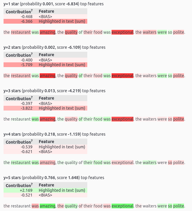
The output of the explain functon should look something like this
You might also want to check the model weights with:
te.explain_weights(target_names=list(model.config.id2label.values()))
ELI5 and a Remotely Hosted Model / API
This one is quite fun and exciting. Since LIME is model agnostic, we can get an explanation for a remotely hosted model assuming we have access to the full probability distribution over its labels (and assuming you have enough API credits to train your local model).
In this example I’m using Huggingface’s inference api where they host transformer models on your behalf - you can pay to have your models run on GPUs for higher throughput. I made this guide with the free tier allowance which gives you 30k tokens per month - if you are using LIME with default settings you could easily eat through this whilst generating a single explanation so this is yet again a contrived example that gives you a taster of what is possible.
Setting up
For this part of the tutorial you will need the Python requests library and we are also going to make use of scipy. You will also need a huggingface account and you will need to set up your API key as described in the documentation.
Building a Remote Model Adapter
Firstly we need to build a model adapter function that allows ELI5 to interface with huggingface’s models.
import json

import requests

MODEL="nlptown/bert-base-multilingual-uncased-sentiment"
API_TOKEN="YOUR API KEY HERE"
API_URL = f"https://api-inference.huggingface.co/models/{MODEL}"
headers = {"Authorization": f"Bearer {API_TOKEN}"}

def query(payload):
    data = json.dumps(payload)
    response = requests.request("POST", API_URL, headers=headers, data=data)
    return json.loads(response.content.decode("utf-8"))

def result_to_df(result):
    rows = []

    for result_row in result:
        row = {}
        for lbl_score in result_row:
            row[lbl_score['label']] = lbl_score['score']

        rows.append(row)

    return pd.DataFrame(rows)

def remote_model_adapter(texts: List[str]):

    all_scores = []

    for text in texts:

        data = query(text)
        all_scores.extend(result_to_df(data).values)

    return softmax(np.array(all_scores), axis=1)
Next we simply run the text explainer using our new model adapter - I artificially limit the samples to a small number so that I don’t wipe out that 30k tokens limit - but remember that doing this will also limit the local fidelity of the model - ideally we want to keep the number quite high.
from eli5.lime import TextExplainer

te = TextExplainer(n_samples=100, random_state=42)
te.fit("""The restaurant was amazing, the quality of their
food was exceptional. The waiters were so polite.""", remote_model_adapter)
te.explain_prediction(target_names=list(model.config.id2label.values()))
Checking whether the explanation is trustworthy
How do we know if our explanations are good? Like any other ML model, the models produced by LIME should be evaluated using a held-out/unseen test set of perturbed examples that have not been seen before. If the local model can do well at predicting the black box weights for other, local examples that it’s not seen yet, then we can assume that the model is a good fit (at least within the specific ’locality’ under analysis).
When we evaluate the local model against the black box model we want to know that, at the very least, the local model is making the same class predictions as the parent black-box model (do both the child model and parent model predict the same most likely class). However, it is also useful to know precisely how similar those outputs are (given that both models predict the same ‘most likely’ class, what is the percentage difference in probability between the two predictions). A good local model should produce a very similar probability distribution to the parent black-box model for the same inputs. Therefore we use KL-Divergence as our performance metric in order to evaluate how well the model is performing. In a nutshell KL-Divergence tells you how similar 2 probability distributions are - and we want this number to be as small as possible (i.e. the probability distributions are pretty much the same).
ELI5 provides this functionality all for free (generates a test set of perturbed examples and evalutes the final model automatically) so all we need is to look at the metrics and interpret them. For any of the above examples you should be able to run te.metrics_ in Jupyter to get an output similar to the one below:
{'mean_KL_divergence': 0.01961629150756376, 'score': 0.9853027527973619}
The score metric is our local model accuracy which is 98.5% - that’s quite reassuring. The mean KL Divergence is low at 0.0196 - this can be interpreted as a mean difference/divergence in the predictions of about 2% across the whole dataset which seems acceptable (although in your use case that might not be acceptable depending on scale, regulatory requirements etc. That’s a call you or your business sponsor have to make).
If these KL divergence is high or the score is low then you have a bad local model and it’s worth checking to see why that might be the case and probably best not to trust the results. The ELI5 Documentation has some excellent information on specific cases where your NLP model might fail and how you might go about diagnosing these issues.
Using Explanations in Practice
Where is it appropriate to use these explanations? Certainly if you’re mid data-science workflow and you want to do some error analysis to see why you’re getting some surprising false-positives or false-negatives then these explanations might be a great place to start.
One elephant in the room is the question of how and when to show these explanations to end users and how to set appropriate expectations. Certainly there is a lot of nuance to interpreting these explanations that should prevent one from hastily drawing conclusions about the far-reaching conclusions (as we discussed above). Therefore if you are planning to allow users to see explanations, some level of training and an informative and clear user experience are going to be key. Given this nuance, I don’t think I’d recommend using explanations in an automated capacity (e.g. workflows that change depending on the outcome of a LIME model) unless it is just to flag something for manual review.
Finally, We should briefly touch on the compute requirements. Every time we ask for an explanation we are fitting (dependant on sample size parameter) a few thousand small models which takes 20-30 seconds on my 2020 laptop. Therefore getting an explanation for one data point is not prohibitive but having one for every decision ever made by a model quickly becomes prohibitive in production environments with 10k+ rows of data (more likely millions of rows). A compromise could be to allow end users request an explanation for specific decisions that they’re interested in on a case-by-case basis. A 30 second wait can be managed through user experience.
Conclusion
In this post I have given you an insight into how LIME works under the covers and how it uses simple local models to offer explanations of more powerful black-box models. I’ve discussed some of the limitations of this approach and given some practical code examples for how you could apply LIME to commonly used frameworks in Python as well as a remote model API.
If you enjoyed this article please take a moment to tweet, toot or send me a webmention.
Replies & Web Activities
If you would like to comment or reply then toot me or bluesky me about this url, or send me a webmention
2 Likes
2 Reposts